Data-Driven Control
Control Theory for humans. The PID controller design based entirely on experimental data collected from the plant.

Please Star me on GitHub for further development.
Table of Contents
PID Controller Example
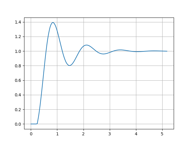
PIDController class can be used directly if the controller gains are already calculated. PIDController class is based on Thread Class. So it can be used as Tread. This features provides fixed PID loop frequency.
from ddcontrol.model import TransferFunction
from ddcontrol.control import PIDController
import numpy as np
import matplotlib.pyplot as plt
import time

#Creates PID controller and test model
pid = PIDController(kp=30, ki=70.0, kd=0.0, kn=0.0)
ref = 1.0
tf = TransferFunction([1.0], [1.0,10.0,20.0], udelay=0.1)

#Control loop
history = []
u = 0.0
pid.start()
start = time.time()
for _ in range(1000):
    t = time.time() - start
    y = tf.step(t, u)
    u = pid.update(ref-y)
    history.append([t,y])
    time.sleep(0.001)

#Stops PID controller
pid.stop()
pid.join()

#Plots result
np_hist = np.array(history)
fig, ax = plt.subplots()
ax.plot(np_hist[:,0], np_hist[:,1])
ax.grid()
plt.show()
Controlled output:
PID optimization for known Transfer Function
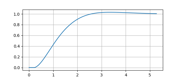
If the transfer function is already known, controller gains can be calculated by pidopt method.
from ddcontrol.model import TransferFunction
from ddcontrol.control import pidopt
import numpy as np
import matplotlib.pyplot as plt
import time

#Creates transfer function
tf = TransferFunction([1.0], [1.0,10.0,20.0], udelay=0.1)

#Optimize PID controller
pid, _ = pidopt(tf)
ref = 1.0

#Control loop
history = []
u = 0.0
pid.start()
start = time.time()
for _ in range(1000):
    t = time.time() - start
    y = tf.step(t, u)
    u = pid.update(ref-y)
    history.append([t,y])
    time.sleep(0.001)

#Stops PID controller
pid.stop()
pid.join()

#Plots result
np_hist = np.array(history)
fig, ax = plt.subplots()
ax.plot(np_hist[:,0], np_hist[:,1])
ax.grid()
plt.show()
Controlled output:
Transfer Function Estimation for unknown SISO system
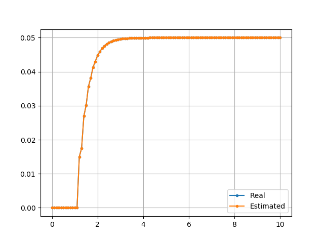
If the transfer function is unknown for system, the transfer function can be estimated by tfest method.
from ddcontrol.model import TransferFunction, tfest
import numpy as np
import matplotlib.pyplot as plt

#Creates a transfer function and input output data
tf = TransferFunction([1.0], [1.0,10.0,20.0], 1.0)
t, y, u = np.linspace(0,10,101), np.zeros(101), np.ones(101)
for index in range(t.size):
    y[index] = tf.step(t[index], u[index])

#Predicts transfer function
tf_est, _ = tfest(t, y, u, np=2, nz=0, delay=True)
y_est = np.zeros(101)
for index in range(t.size):
    y_est[index] = tf_est.step(t[index], u[index])

#Plots result
fig, ax = plt.subplots()
ax.plot(t, y, '.-', label='Real')
ax.plot(t, y_est, '.-', label='Estimated')
ax.legend()
ax.grid()
plt.show()
Step response of real system and estimated system:
ddcontrol.control module
Created on Thu Jan 9 20:18:58 2020
@author: eadali
-
class
ddcontrol.control.PIDController(kp, ki, kd, kn, freq=10.0, lmin=-inf, lmax=inf)[source]¶ Bases:
threading.ThreadAdvenced PID controller interface.
Parameters: Example
>>> from ddcontrol.model import TransferFunction
>>> from ddcontrol.control import PIDController
>>> import numpy as np
>>> import matplotlib.pyplot as plt
>>> import time
>>> #Creates PID controller and test model
>>> tf = TransferFunction([1.0], [1.0,10.0,20.0])
>>> pid = PIDController(kp=30, ki=70.0, kd=0.0, kn=0.0)
>>> ref = 1.0
>>> #Control loop
>>> pid.start()
>>> y, u = np.zeros(900), 0.0
>>> start = time.time()
>>> for index in range(y.size):
>>>     t = time.time() - start
>>>     y[index] = tf.step(t, u)
>>>     u = pid.update(ref-y[index])
>>>     time.sleep(0.001)
>>> #Stops PID controller
>>> .stop()
>>> pid.join()
>>> #Plots result
>>> fig, ax = plt.subplots()
>>> ax.plot(y)
>>> ax.grid()
>>> plt.show()
-
run()[source]¶ Method representing the thread’s activity.
You may override this method in a subclass. The standard run() method invokes the callable object passed to the object’s constructor as the target argument, if any, with sequential and keyword arguments taken from the args and kwargs arguments, respectively.
-
-
ddcontrol.control.pidopt(tf, end=10.0, wd=0.5, k0=(1.0, 1.0, 1.0, 1.0), freq=10.0, lim=(-inf, inf))[source]¶ PID optimization function for given transfer function
Parameters: - tf (TransferFunction) – TransferFunction object for optimization.
- end (float, optional) – Optimization end time
- wd (float, optional) – Disturbance loss weight [0,1].
- k0 (tuple, optional) – Initial PID controller gains.
- freq (float, optional) – PID controller frequency.
- lim (tuple, optional) – Output limit values of PID controller
Returns: Optimized PIDController and OptimizeResult.
Return type: Example
>>> from ddcontrol.model import TransferFunction
>>> from ddcontrol.control import pidopt
>>> #Creates transfer function
>>> tf = TransferFunction([1.0], [1.0,10.0,20.0], udelay=0.1)
>>> #Optimizes pid controller
>>> pid, _ = pidopt(tf)
>>> print('Optimized PID gains..:', pid.kp, pid.ki, pid.kd, pid.kn)
ddcontrol.model module
Created on Wed Jan 15 10:06:42 2020
@author: ERADALI
-
class
ddcontrol.model.StateSpace(A, B, C, D, delays=None)[source]¶ Bases:
objectTime delayed linear system in state-space form.
Parameters: - B, C, D (A,) – State space matrices
- delays (array_like, optional) – Delay values
-
class
ddcontrol.model.TransferFunction(num, den, udelay=None)[source]¶ Bases:
ddcontrol.model.StateSpaceTime delayed linear system in transfer function form.
Parameters: - den (num,) – Numerator and denumerator of the TransferFunction system.
- udelay (float, optional) – Input delay value
-
ddcontrol.model.tfest(t, y, u, np, nz=None, delay=False, xtol=0.0001, epsfcn=0.0001)[source]¶ Estimates a continuous-time transfer function.
Parameters: - t (float) – The independent time variable where the data is measured.
- y (float) – The dependent output data.
- u (float) – The dependent input data.
- np (float) – Number of poles.
- nz (float, optional) – Number of zeros.
- delay (bool, optional) – Status of input delay.
- xtol (float, optional) – Relative error desired in the approximate solution.
- epsfcn (float, optional) – A variable used in determining a suitable step length for
- forward- difference approximation of the Jacobian (the) –
Returns: Estimated TransferFunction and covariance ndarray
Return type: Example
>>> from ddcontrol.model import TransferFunction, tfest
>>> import numpy as np
>>> #Creates a transfer function and input output data
>>> tf = TransferFunction([1.0], [1.0,10.0,20.0])
>>> t, y, u = np.linspace(0,10,101), np.zeros(101), np.ones(101)
>>> for index in range(t.size):
>>>     y[index] = tf.step(t[index], u[index])
>>> #Predicts transfer function
>>> tf, _ = tfest(t, y, u, np=2, nz=0)
>>> print('Transfer function numerator coeffs..:', tf.num)
>>> print('Transfer function denumerator coeffs..:', tf.den)
ddcontrol.integrate module
Created on Thu Feb 6 22:05:52 2020
@author: eadali
-
class
ddcontrol.integrate.CInterp1d(x0, g, lsize=10000.0)[source]¶ Bases:
objectA conditional interpolation function interface.
This class returns a value defined as y=g(x) if x<x0, else interpolate(x)
Parameters:
-
class
ddcontrol.integrate.dde(f)[source]¶ Bases:
ddcontrol.integrate.odeA interface to to numeric integrator for Delay Differential Equations. For more detail: Thanks to http://zulko.github.io/
Parameters: f (callable) – Right-hand side of the differential equation.
-
class
ddcontrol.integrate.ode(f)[source]¶ Bases:
objectA generic interface class to numeric integrators. Solve an equation system \(y'(t) = f(t,y)\).
Parameters: f (callable) – f(t, y, *f_args)Right-hand side of the differential equation. t is a scalar,y.shape == (n,).f_argsis set by callingset_f_params(*args). f should return a scalar, array or list (not a tuple).